Aggregate demand

Aggregate demand Is the total amount of spending on goods and service in a period of time at a given price level. AD is quantitatively the same as GDP in the long run.

What affects aggregate demand? 

As GDP and AD are equal the same thing which affect GDP also affect AD.

$AD = C +I\hspace{0.17em}+\hspace{0.17em}G\hspace{0.17em}+(X-M)$

So by looking at the formula the following factors affect AD:

1. Consumption
2. Investment
3. Government spending
4. Net exports.(X-M)

Causes of changes in consumption affecting Aggregate demand

Note: In the below table, the change is always increase in a factor, to show the direction of the effect this change has on AD.

For a decrease, the effect will be the opposite. 

Change	Why this affects AD (positively)
Increase in income	increases the amount you have to spend.
Increase in wealth	An increase in your personal assets makes people more likely to spend as they aren't under pressure to save.
Increase in consumer confidence or expectations	If you expect that in the future you will have more to spend you will not save for the future, you will spend in the moment
Decrease in household indebtedness	Lower debt increases households want to spend as they don't have to worry about falling further in debt.
Decrease in interest rates	If it costs less to borrow money from the bank, you will borrow more, and hence spend more.  Interest rates on banks will also go down, so you are less inclined to save and hence take your money out the bank and spend it..

Higher interest = lower consumption

Lower interest = higher consumption

Causes of changes in investment affecting Aggregate demand

Taking out loans leads to investment because people use the money to buy investments for the future like factories, buying shares or houses. 

A mortgage is an example of a loan which leads to an investment. 

Change	Why this affects AD (positively)
Decrease in interest rates	The lower the interest rates on loans, the more loans firms will borrow, as they can afford to do so. They will then invest it.
Increase in national income level	The more income the more you take out loans. Which leads to investment.
Advances in technology.	When technology advances all companies will want to invest in it to stay competitive in the market.
Business confidence or expectations of the future.	if a firm is more confident or expects higher demand in the future they will be more likely to make large investments, which they thing will pay off.

Demand side policies affecting aggregate demand

Demand side policy: a government policy affecting AD

Fiscal policy: A policy which changes government spending and/or taxation rates. 

Monetary policy: An official policy governing the supply of money and the interest rates in the economy 

if a firm is more confident or expects higher if a firm is more confident or expects higher

Policy	Change	Effect on AD
Expansionary fiscal policy	Decrease personal income tax	Households spend more, as they have more to spend
	Decrease in corporate tax	Firms spend more, as they have more to spend
	Increase in government sending	Government spending is one of the variables in GDP, so this increases economics activity
Contractionary fiscal policy	opposite of expansionary	opposite of expansionary
Monetary fiscal policy	Increase in base interest rate	More expensive to invest, so less investing.

Aggregate supply

Total amount of good and services produced by all industry in an economy in a given time period. 

Short-run aggregate supply (SRAS)

short run aggregate supply is when one factor of product remains fixed.

SRAS diagram:

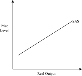
What affects SRAS?

• Wages
• Taxes
• Cost of raw materials

Keynesian vs New classical belief

Keynesian belief: The keynesians believe that intervention form the government is necessary and the government should intervene during periods of low economic activity

New classical belief: The market forces are efficent to deal with all problems and thus there should be minimal or no intervention from the government. All problems will sort themselves out with enough time.  

Long-run aggregate supply (LRAS) 

This depends on whether you agree with keynesian or new classical ideas. 

1. From a new classical point of view, resources are already being used at a maximum potential so real output will stay the same no matter what happens to aggregate supply. Only price level will change. hence the graph is perfectly inelastic. 
2. From a Keynesian point of view, there is a section of the GDP level where increasing aggregate supply, real output will increase with no change in price, then after a point price begins to change. 

Full employment

The full employment level of output is produced when all factors of production are fully employed by the economy(the rate of employment is equal to the natural rate of employment). The equilibrium level of output is the level of output produced at the intersection of aggregate demand and short-run aggregate supply, and may be below or above the full employment level. 

Inflationary gap

An inflationary gap is a macroeconomic concept that describes the difference between the current level of real gross domestic product (GDP) and the anticipated GDP that would be experienced if an economy is at full employment. 

These gaps are shown in the short-run if aggregate demand increases.

New classical

An increase in real output is possible in the short-run even if it is not possible in the long run.

However in the long run this level of output always returns to the same as before however now at a higher price level.

1. AD shifts right because of demand side policies. Workforce has to work overtime in the short run to demand so it is possible. 
2. However, they can't supply that level of demand forever, it is not sustainbale. So supply curve shifts left, in the long run.
3. The equilibrium level is now vertically above the old one. Price level is now higher, but the level of output is the same.

Keynesian

An increase in real output is possible in the long run but there is a point where it becomes the same as new classical, on the vertical line part of the LRAS curve. At this point a shift in AD, does not change real output.

Supply side policies

Please see the supply side section of "Economic Policies"

https://ibrecap.com/DP/Economic%20Policies#20 

The Multiplier Effect

A phenomenon whereby a given change in a particular input, such as government spending, causes a larger change in an output, such as gross domestic product.

Marginal Propensities

Percentage of every extra unit of income which consumers are inclined to spend on a certain thing. 

MPC: Marginal Propensity to Consume. Percentage of extra income which goes into consumption

MPS: Marginal propensity to Save. Percentage of extra income which is saved.

MPM: Marginal Propensity to Import. Percentage of extra income which is spent on imported goods.

MRT: Marginal Rate of Tax. Percentage of extra income taken by tax.

MPW: Marginal Propensity to Withdraw. Total amount of extra income not spent on consumption.

Formulas for Marginal propensities

MPS + MPM + MRT = MPW

MPC + MPW = 1

Note: MPC + MPW is 1 because a consumer either spends their money on consumption or doesn't. Since MPW represents money not spent on consumption, MPC + MPW should be equal to 100% of their extra income.

The multiplier effect in action

Imagine the government spends $1 million  on building a bridge. Where MPC = 0.6. (So, 60% of extra income goes into consumption)

Phase of multiplier effect	Who receives extra income?	Percentage of  original money spent
Government spends money to make bridge	Construction Workers Managers Engineers Cement Steel Asphalt ect…	100%
Workers and businesses use this money to spend it on extra things they want, but don't need. They spend 60% because the MPC is 0.6.	Extra food Houses Cars Clothing	60%
The people who sold the items to the workers and businesses now have a little bit of extra income, to spend on things.	Same as before.	60%*60% = 36%
This repeats with the extra income of the the next phase, always being 60% of the extra income gained in the previous phase. If you add together the incomes of each phrase the percentage you get is 150% which means more money is spent then the original government spending!

Calculating the extra output from multiplier effect

The pattern is to multiply the previous phase's extra income by 60%, to get the next phase extra income. 

If you remember from Maths, this is an example of a geometric series.

The percentage of input spent on consumption of at phase p is given by: $C_p=MP{C}^p$ where.

Therefore based on infinite geometric series the extra output or multiplier is given by:

$Multiplier = \frac{1}{1-MPC}$

Since 1-MPC is just MPW, the multiplier is also given by:

$Multiplier = \frac{1}{MPW}$

Example of calculating the multiplier effect

Government spending = $50

• MPS = 0.15
• MPM = 0.1
• MRT = 0.2

1. Formula: MPW = MPS + MPM +MRT
2. To calculate MPW add together all components of withdrawal
   • MPW = MPS + MPM + MRT
   • MPW = 0.45
3. Insert value for MPW into the multiplier formula, and evaluate
   • $Multiplier = \frac{1}{MPW}$
   • $Multiplier = \frac{1}{0.45}=2.2\dot{2}$
4. Multiply the multiplier by the input to get the output
   • Output = 50*2.22
   • Output = $111

 

 

 

View count: 7785